As it can be easily seen, since (1) α₁(t) is formulated as a difference equation, and there are (2) serial correlations, and (3) multicollinearity, in the proposed model, direct application of ordinary least squares estimation, to find parameter, is hard to apply and the estimated parameters cannot be efficient estimators.

Thus, another approach, which is originally presented by Kalman(1960) and Harvey(1981, 1986), is taken.

1. Operationalizations

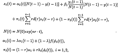
The main equations need to estimate, are;

where, definitions are same as previously given.

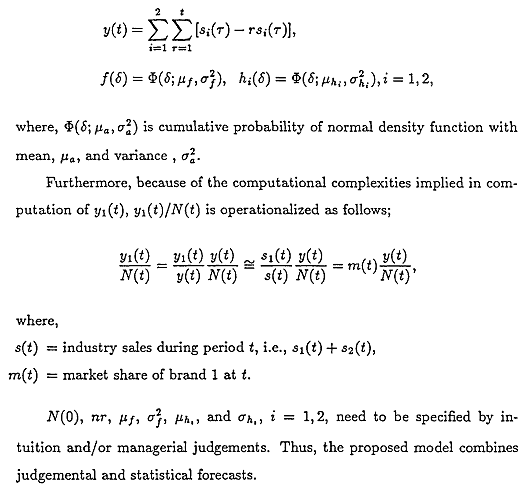
To estimate parameters for a proposed model, some additional equations are need such as;

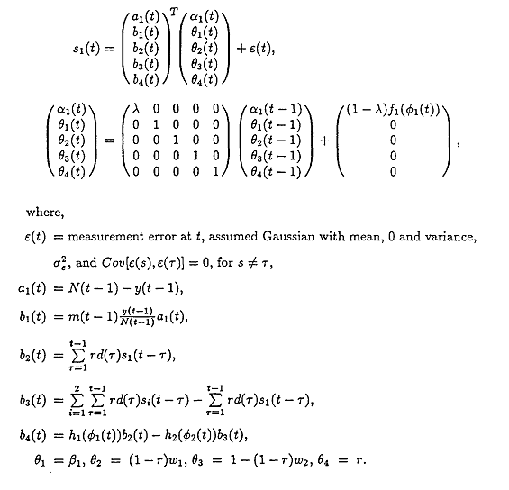
To apply Kalman filter to the proposed model, the above equations are operationalized as follows;

2. Kalman Filter and Likelihood Function

Kalman updating equations for the previously operationalized equations are known from optimal control theory literature(Meditch 1969, Anderson and Moore 1971). Define,

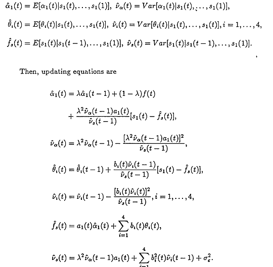
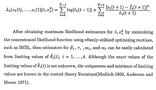
Using prediction error decomposition method(Harvey 1981, 1986), the concentrated likelihood function becomes;

3. Forecasting

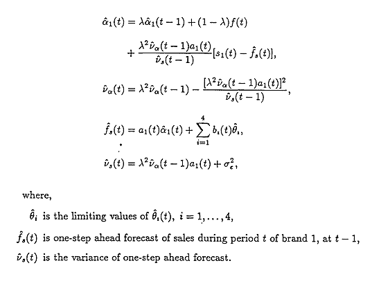
After obtaining all the necessary parameters, the last work remained is how to forecast future sales using the estimated parameters. We can also use Kalman forecasting equations to predict future sales;