1. Adoption-Sales Submodel

This section introduces a model which, is developed using an initial-purchase framework in a duopolistic competition to predict company sales of a durable good.

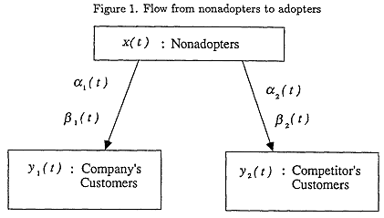
Let the number of people in the target market, N(t), assumed varying over time, i.e., dynamic saturation level, be divided into x(t)-the number of potential customers who have not yet adopt the product, y₁(t)-the number of customers who are using company brand, and y₂(t)-the number of customers who are using competitors' brands. By definition,

x(t) + y₁(t) + y₂(t) = N(t).

The variables x, y₁, y₂ represent states in a diffusion process. At any point in time) a consumer will be in one of these states.

Figure I describes a flow model of a process, comprising three states, (1) nonadopters, (2) company customers, and (3) competitors' customers.

One variable, influencing the movement of nonadopters from x to y₁ or y₂ for a new product, is the information acquired from. contact with prior purchasers, i.e., word-of-mouth. Early adopters of a new product or new idea interact with less innovative members of the group. The potential adopters may be influenced in their purchase timing by the early adopters of the product.

Also a certain proportion of potential customers may purchase the product independently of the influence of word-of-mouth. This inducement to purchase will represent the effects of distribution, promotion) advertising, and other forms of marketing efforts. These two factors, influencing diffusion of new product, originally modeled by Bass(1969). Bass model also implies customer dichotomization between innovators and immitators.

(1) Word-of-mouth effect

The imitation effect, originally modeled by Bass(1969), interpreted as

word-of-mouth effect at t
= ( immitation rate constant )
X ( the percentage of adopters to total market size at t ) .

Bass model and its extensions imply the effectiveness of each adopter to nonadopter to try a new product, β(t), is the product of a coefficient of β, assumed to be constant over time, and a proportion of adopters to total market size.

To represent competitive phenomena) we need to adjust the above model to consider company specific word-of-mouth effect. Thus, the word-of-mouth influence is modeled as follows;

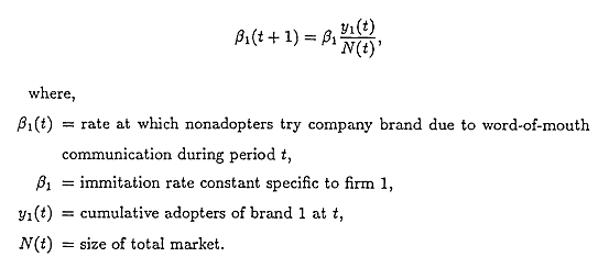
Here, we take a view, which seemingly similar to original Bass model, that the rate of diffusion by word-of-mouth at t is the product of two terms - the percentage of current company customers to total market size at t-1, and an individual imitation rate constant.

And, furthermore, we should consider an word-of-mouth effect come from competitors' customer stock, i.e., the interaction effect between company and competitors' brands' using groups.

With some manipulations and slight different interpretation, we don't need to include and formulate this interaction effect explicitly. The rationale why the above equaton, implicitly, include an word-of-mouth effect from a competitors' customer stock, i.e., an intergroup communication effect on adoption-sales, can be explained as follows. If there is no intergroup communication, then,

β(t) = β₁(t) + β₂(t),

where,

β(t) = the rate at which nonadopters try the product due to word-of-mouth effect, irrelevant of brand,

β_i(t) = word-of-mouth effect of trying brand _i, _i = 1,2.

If there is an intergroup communications, then a simple sum of β₁(t) and β₂(t) is not equal to β(t), since there must be an interaction term which represents the influence of intergroup communication. This interaction effect can not be easily formulated and usually this interaction effect is small relative to word-of-mouth effect from company customers. This may be a reason why researchers, modeling diffusion process in an oligopoly framework, do not model the intergroup communication explicitly. Now)

β(t) = β₁(t) + β₂(t) + interaction term between two brands at t.

By some manipulations, we can include interaction effect between two groups β(t) into β₁(t), i.e.,

β₁(t) = β(t) + β₂(t) - interaction term except β₁(t) at t.

Since we don't know the exact form of the right hand side of the above equation, and β₁(t) implicitly includes β(t), β₂(t) and interaction term at t, we can use β₁(t) as an imitation effectiveness rate, and this β₁(t) gets different meaning.

(2) Marketer-controls

Bass(1969) originally modeled based on a premise that an innovation rate is constant over time. But, this assumption has been relaxed by many researchers, as previously cited. It is assumed here that

(1) marketing expenditures affect the present and future demand for the new product and, hence, marketing efforts accumulate some kind of capital(goodwill), and, furthermore,

(2) this capital depreciates over time by forgetting and competitive marketing efforts.

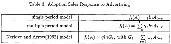
Simon and Sebastian(1987) compared three types of advertising expenditures' effectiveness, - single period model, multiple period model, and Nerlove and Arrow(1962) model, as given in table 3, in a diffusion framework. Their research support an Nerlove and Arrow model.

Following Nerlove and Arrow(1962), it is supposed that

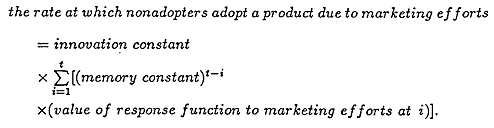
Since the main focus of this paper is to design a forecasting model, the desirable property of a model is adaptive, i.e., model can be adjusted as new information is acquired(Little 1970).

Thus, the best alternative is a difference equation form which strictly has properties of Nerlove and Arrow(1962) model.

Following Friedman(1971) and Little(1975), adoption-sales response function to marketing efforts is modeled as follows;

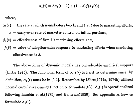
Another interpretation for λ, may be possible. If a firm is in competitive environments, carry-over rate might represent the degree of the competition, since the effectiveness of marketer control on future initial-sales will be diminished by competitors' marketing actions, as well as forgetting. This assertion may be controversial, but it is not an absurd interpretation. Most firms spend much money on marketing actions continuously - rather than pulsing - by this reason.

(3) Synthesis

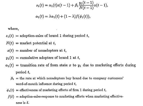
Combining previously mentioned contents gives two separable equations;

2. Replacement-Sales Submodel

According to the marketing literatures(Hughes 1973, Lilien and Kotler 1983, Kotler 1989), sales estimation methods and marketing strategy depend on whether managers deal with a one-time purchased product, an infrequently-purchased product, or a frequently-purchased product. Figure 2(a) illustrates the product life cycle that can be expected for just one-time purchased products.

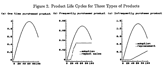
Frequently-purchased products such as coffee and soops, have product life cycle resembling Figure 2(b). Infrequently-purchased products such as automobiles, computers, and washing machines, exhibit replacement cycles - see Figure 2(c), - dictated either by their physical wearing out or their obsolescence with changing styles, features, and tastes.

Thus, sales-forecasting methods should be different whether which products we want to forecast.

Fortunately, in contrast to nondurables, the repeat-purchasing trends of durables, can be approximated by a functional form, called as a replacement distribution.

If customers have an opportunity to switch the brand, it is desirable to include this behavior in a model as a brand-switching ratio or other reasonable parameters.

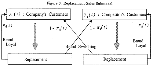
Hence, we can think that a good parametrization of replacement distribution and brand switching will give birth to suitable model to account for replacement-purchasing behavior. Figure 3 shows the replacement-sales submodel.

(1) Replacement distribution

If we define replacement demand as a demand which is motivated by "the replacement of an old unit not performing according to the household's requirements," then we can think that replacement sales is influenced by (1) product's age - while this factor may dominate the replacement rate, the replacement of a durable good is also affected by a multitude of following random factors, (2) overload(underload) - very heavy(light) use of a product which advances(delays) the replacement probability determined by its age, (3) percent of owners who will replace - the propensity of consumers to replace when new product is launched, (4) practicality of repair vs. replacement (Harrell and Taylor 1981).

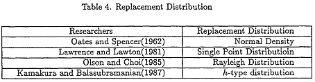
Four types of replacement distribution have been published in a diffusion framework(Chung and Park 1988).

Lawrence and Lawton(1981) have proposed a simple model of replacement purchases in which the service life of the durable is assumed to be constant and known a priori.

Gates and Spencer(1962) specified a replacement rate function by normal density distribution.

Olson and Choi(1985) model utilizes the Rayleigh distribution to model replacements, and recognizes that the product life is not constant but stochastic.

More recently, Kamakura and Balasubramanian(1987) have extended the Olson and Choi model. They used h-type replacement distribution, initially presented by Kimball(1947).

Functional forms, presented by Olson and Choi and Kamakura and Bal-asubramanian are given in appendix B.

Kamakura and Balasubramanian model, only, satisfies above four cited factors that can impact replacement demand. Thus) replacement distribution is modeled utilizing h-family distribution.

Table 4 summarizes the above replacement distributions.

(2) Brand switching

The proportion of brand loyal customers is assumed to be dynamic and influenced by two mutually exclusive factors, one is marketer controllable factor, and the other, uncontrollable factor.

Marketer uncontrollable portion of brand-choice decision is assumed to be constant, since this part of consumer behavior is determined by the psychological aspects - internal inertia, not influenced by external cues such as promotion, advertising, and price discount.

Lilien(1974a, 1974b), Jones and Zufryden(1980, 1982), and Hauser and Wisniewski(1982) presented insights how to include consumer response to marketing variables into stochastic brand-choice models.

Marketing efforts may affect attitude and attractiveness of consumers, toward the products, positively and negatively - the sign of direction is a controversial issue in marketing(Little 1979), hence, consumer's brand choice decision is assumed to be influenced by marketing mix variables, as well as internal inertia.

To accommodate interactive - intrafirm and interfirm - nature of marketing mix variables, the same constructs as given by Lambin et al.(1975) and Hanssens(1980) are utilized.

Then, the brand-loyal ratio of firm i during period t is

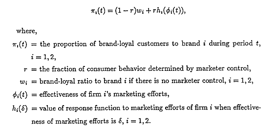
If marketer control has no effect on brand choice, r = 0 in the above equation. If consumer behavior can be completely manipulated by marketer control, then r = 1.

(3) Synthesis

The replacement sales of firm 1, is composed of two parts, one is a demand from customers using company brand, who show brand loyalty, the other demand comes from customers using competitors' brands. Then, replacement sales of firm 1 is

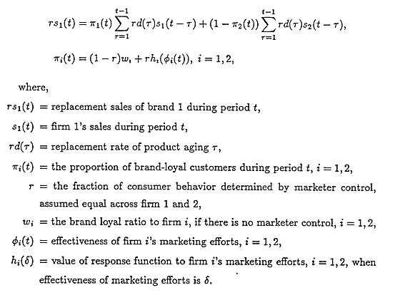
Note that the above representations of diffusion process has some restrictive assumptions about,

(1) rd(t) ; that is, replacement distribution for products between two brands are exactly same, and

(2) r ; that is, the fraction of consumer behavior in brand choice determined by marketer control are same between two brands.

But, it can be easily seen that these assumptions are not absurd.

3. Combining the Two Models

(1) Full model

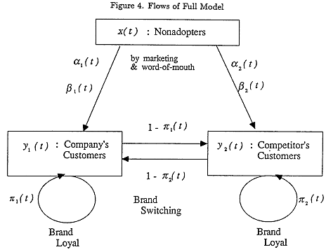
This section integrates the above two sections and gives a diffusion model which integrates a replacement demand and marketing mix variables for two firms introducing competing brands of a new durable product.

Figure 4 represents the flow of this full model.

The following equations are full model considered;

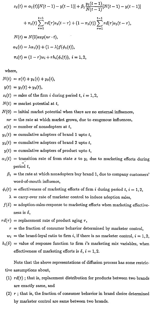
(2) Assumptions

The assumptions, implicitly or explicitly made, of the proposed model will be summarized, here;

(1) There are only two firms in the market, i.e., duopoly market. Extensions to an oligopolistic market is straightforward if we divide competitors into several firms.

(2) Market potential is growing due to economic growth and price reduction.

(3) Ownership of multiple units of the product is negligible and all scrapped

units are immediately replaced.

(4) Replacement rate for products is assumed equal for all brands. This

assumption implies two premises, product and consumer homogeneity.

(5) Potential adopters of an innovation are influenced by two means of communication - mass media and word-of-mouth. ^

(6) The adopters of an innovation comprise two groups - innovators and imitators.

(7) An intrafirm, as well as interfirm interactions between marketing mix

variables, exist.

(8) Marketing efforts creates and accumulates some kind of capital(goodwill)

and this capital depreciates over time.

(9) Consumer response functions to marketing efforts are dynamic because

of dynamic marketing efforts and dynamic competition effects.

(10) Consumer responses to marketing efforts are different between trial and

repeat-buying decision.

(11) Brand choice decision in replacement purchasing is influenced by two

factors - marketer controllable factor, and uncontrollable factor.

(12) The fraction of consumer behavior in brand choice, influenced by marketing efforts, are equal for all brands.